Section 7.6: Time Evolution

The Schrödinger equation in one dimension,

[−(ħ²/2m)∂²/∂x² + V(x)] ψ(x,t) = iħ(∂/∂t) ψ(x,t),                   (7.7)

governs the time evolution of quantum mechanical systems. We can also write this equation in terms of the Hamiltonian operator, H = [−(ħ²/2m)∂²/∂x² + V(x)] , as

Hψ(x,t) = iħ(∂/∂t) ψ(x,t),                   (7.8)

The left-hand side of the Schrödinger equation involves just the spatial part of ψ(x,t), and for energy eigenstates we can determine how the spatial part behaves from the time-independent Schrödinger equation. The right-hand side just involves the temporal part of ψ(x,t).

For energy eigenstates, Hψ(x) = Eψ(x), and from the Schrödinger equation the time development of such a state is

ψ(x) = e ^−iEt/ħ ψ(x)                   (7.9)

while for states in general we have

ψ(x,t) = e^−iHt/ħ ψ(x,t)                   (7.10)

where e^−iHt/ħ is called the time-evolution operator, U_T(t).⁹

Looking at Eq. (7.9), it is clear that time-dependent states will be complex. How do we represent such complex functions? We will demonstrate two possible representations. Consider an arbitrary complex wave function that we choose to write as:

ψ(x,t) = ψ_Re(x,t) + iψ_Im(x,t)                    (7.11)

where we can show the real (blue) and/or imaginary (pink) parts of the wave function. Conversely, when you check the box and "set the state," we can write the wave function as

ψ(x,t) = A(x,t) e^iθ(x,t)_,                   (7.12)

where we have chosen to write all of the complex behavior in the exponential.  When we do this, the angle, θ(x,t) = tan⁻¹[ψ_Im(x,t)/ψ_Re(x,t)] is called the phase of the wave function. The real part of the wave function in this representation is just the probability amplitude A(x,t) = [ρ(x,t)]^1/2.  How do we show the wave function in this amplitude and phase description? We will depict the amplitude of the wave function as the magnitude of the distance from the bottom to the top of the wave function at a given point and time. 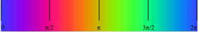We represent the phase as the color of the wave function. The color strip above the animation shows the map between phase angle and color. Since quantum-mechanical time evolution involves a minus sign in the exponential, the phase evolves in time clockwise in the complex plane.

Explore the time dependence of the energy eigenstate of a particle in an infinite square well by changing state and representation.  In the animation the time is given in terms of the time it takes the ground-state wave function to return to its original phase.  Restart.  For energy eigenstates, the amplitude does not change with time and time evolution just changes the overall phase of the wave function.  As a consequence, energy eigenstates are also called stationary states.

If there is a time-dependence, we can write the expectation value of an operator as¹⁰

<A> = ∫ ψ^*(x,t) A ψ(x,t) dx =   ∫ ψ^*(x) e^iHt/ħ  A e^−iHt/ħ ψ(x) dx          [integral from -∞ to +∞]                    (7.13)

and take a time derivative to find:

d<A>/dt = <∂A/∂t> + i/ħ <[H, A]>.                   (7.14)

In general, if a Hamiltonian has a potential V(x) that is just a function of x, we find that:

d<x>/dt = <p>/m,     d<p>/dt  = −<dV(x)/dx>,     and    d<H>/dt = 0.                   (7.15)

For the special case of a vanishing potential energy function, we find that:

d<p>/dt  = 0.                   (7.16)

All of these relationships are described by Ehrenfest's principle, a statement of the quantum-mechanical (on average) and classical correspondence of dynamical variables.

___________

⁹In general, for an operator O, we know that O ⁻¹O = 1.  For unitary operators O^†O = 1.  In other words, for unitary operators, their inverse is their adjoint.  So for example, the time-evolution operator, U_T, is a unitary operator because [e^iHt/ħ ]⁻¹ = [e^iHt/ħ]^† and therefore U_T⁻¹ U_T = 1.  This is the case as long as H is a self-adjoint or Hermitian operator, which it must be to yield real energies.
¹⁰We can think about a situation where the operators have the time-dependence, but the states do not: ψ_H(x) = e^iHt/ħ ψ_S(x,t) and A_H(t) = e^iHt/ħ A_S e^−iHt/ħ.  This is called the Heisenberg picture.  This is equivalent to the situation where the operators have no time dependence but the states do, which is called the Schrödinger picture.  The difference between pictures amounts to how you decide to group U_T and U_T^† in the expectation value: with the states or with the operator.

© 2006 by Prentice-Hall, Inc. A Pearson Company