A Stewart platform is a mechanical device with six actuators mounted on a level surface in three pairs, crossing over to three mounting points on a top plate. Devices placed on the top plate can be moved in all of the six degrees of freedom in which it is possible for a freely-suspended body to move. These are the three linear movements x, y, z (lateral, longitudinal and vertical), and the three rotations pitch, roll, & yaw. Because the motions are produced by a combination of movements of several of the jacks, such a device is a type of parallel manipulator.
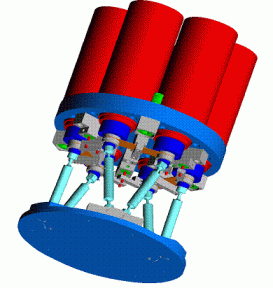
Because the device has six legs, it is often also known as a hexapod (six legs), originally a trademarked name by Geodetic Technology.
In the typical configuration a) the actuators constitute the hexapod legs, but many other configurations are possible such as the figure b) where the actuators are all parallel to each other and push/pull the six legs, or c) and d) in which three actuators act along the main longitudinal axis of the device and the other three act in a plane normal to this axis.
Hexapod kinematics is often described in papers by analytical models of various and sometimes extravagant complexity. In fact, regardless of the particular configuration, the hexapod kinematics can be described by a simple and general mathematical approach.
Inverse kinematics
The objective of the inverse kinematic calculation is to compute the six displacements ΔDi of the actuators required in order to achieve a desired motion of the mobile part:
ΔDi = f (Δx Δy Δz Rx Ry Rz) [1]
Let us define the desired displacement of the mobile part u =(Δx Δy Δz Rx Ry Rz) with respect to a zero position in terms of the homogenous transformation matrix R (4x4) relative to the system references axes. The homogenous transformation method and the computation of the matrix are described in several books on robotics and serial links in particular.
Let us set the matrices PF (6x3) and PM (6x3) with the coordinates (x,y,z) of the virtual hinge points of the leg hinges in the given zero position, respectively attached to the fixed (PF) and to the mobile part (PM). PM and PF must be referenced to the system of axes in which the hexapod motion is to be evaluated.
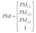
Consider the leg i and define the vector PMi where the first 3 terms of PMi are the x,y,z coordinates of the hinge point and the fourth term is 1:
The positions of the mobile part hinges after the displacement are computed as:
PMinew = R x PMi
where the first 3 terms of PMinew are the x,y,z coordinates of the moved hinge point.
When these coordinates are known the calculation of the actuator displacements is generally straightforward, although the relationship will depend on the particular hexapod configuration. For instance for the configuration illustrated by the figure above, the base points PF can only move in axial direction (z), the actuator displacement ΔZi are computed from the condition that the leg lengths L between the hinges remains constant:
ΔZi = PMinew(3) - PFi,3 + D,
where

Linear approximation
By setting very small displacements, one degree of freedom at the time, one can obtain a linear transformation matrix T with which actuator displacements can be estimated as:
ΔDi = u x T
The matrix T can be inverted and hence a linear approximation to the forward kinematics can be obtained by:
u= ΔDi * T -1 [2]
Forward kinematics
The forward (or direct) kinematics calculation is used to evaluate the position of the mobile part from the knowledge of the six actuator displacements:
(Δx Δy Δz Rx Ry Rz) = f (ΔDi )
The search for an analytical solution is generally futile, but a numerical solution is easily found by solving the implicit equation [1] by an iterative method to compute the zero of
ΔDi - f (Δx Δy Δz Rx Ry Rz) = 0
When the initial approximation is taken by equation [2], the iteration converges very rapidly to the exact solution.